2026-09-05 The OxCaml Type system
As promised, this post is finally up and has a section by section explanation of the OxCaml type system - the typing rules, what type contexts are made up of, the steps taken for inferring modes and the differences between the declarative and the syntax-directed rules of the type system. These topics cover sections 3 and Appendix B of the paper. I wanted to add bits from section 4 (store semantics) and 5 (conversion to a graded call-by-value calculus) but they are substantial parts in themselves and best kept for later.
I hope having working code samples makes this post easy to understand parts of the paper and mentally put together all the pieces that make up the type system. I have tried to keep the accompanying explanations as simple as possible while keeping all the relevant details.
A note on all the code presented in this post: Every block in the post is a
verified toplevel transcript (captured by piping the exact same code through
ocaml -noprompt in a switch with OxCaml 5.2). The code has also been verified
with OxCaml 5.4. The types/values/errors/line numbers/column numbers
are actual outputs from running these blocks. I have gathered all samples at
OxCaml modes code. Feel
free to download it and run the file locally if you wish.
If you would rather not install OxCaml locally first,
Dox is an online
playground where you can copy and paste the OxCaml code blocks and have them
run.
Locks for Closures #
Recall that closures are functions that capture something from their surrounding contexts — variables, values (lists, records, …), references etc. — and types in OxCaml for contexts and variables are: (from the previous post):
Γ ::= ∅ | Γ, x : − | Γ, x : τ @ μτ ::= 1 | τ + τ | τ × τ | □^ν τ | τ @ μ → τ @ μ | ♣A closure with type τ @ μ → τ @ μ capturing a variable with type τ @ μ from
it’s surrounding environment has to ensure that the mode μ of the variable is
acceptable to the closure’s input type μ. A few rules that hold everywhere:
With the third axis of a mode triple ( , , ) being locality and the sub-moding rule (
GLOBAL < LOCAL) - the of the captured variable needs to be the sub-mode of the closure’s . Aglobalvalue can be used in alocalclosure, never the other way around. So global closures cannot contain local variables as the local variables might “escape” their region via the global closure being run in another region.With the first axis of a mode triple ( , , ) being affinity and the sub-moding rule (
MANY < ONCE), the of the captured variable needs to be the sub-mode of the closure’s . Variables marked withmanycan be used in closures markedonce.
Γ,🔒_μ denotes what a closure of mode μ = (a₂,u₂,l₂) is allowed to capture
from its surrounding region. For the second axis, uniqueness, the type system
needs to ensure that unique variables are not captured by closures marked
many. For this the dagger operation for linking unique values that should
only be called once is defined as:
ONCE† := UNIQUE, MANY† := ALIASEDThe join of the uniqueness
for an input variable (on the right hand side
above) and the resulting daggered affinity ONCE†/MANY† creates an updated
value for the uniqueness
of the variable that is captured. Note it
is not the affinity of the capturing closure,
that is being affected, but
the uniqueness of the captured variable driven by the closure’s own daggered affinity.
For easy reference, here’s the join (∨) on each axis directly — the
least upper bound of two values on that axis:
Affinity (MANY < ONCE) #
| ∨ | MANY | ONCE |
|---|---|---|
| MANY | MANY | ONCE |
| ONCE | ONCE | ONCE |
Uniqueness (UNIQUE < ALIASED) #
| ∨ | UNIQUE | ALIASED |
|---|---|---|
| UNIQUE | UNIQUE | ALIASED |
| ALIASED | ALIASED | ALIASED |
Locality (GLOBAL < LOCAL) #
| ∨ | GLOBAL | LOCAL |
|---|---|---|
| GLOBAL | GLOBAL | LOCAL |
| LOCAL | LOCAL | LOCAL |
Each axis’s join operation that is defined over its own two-element order
collapses the result towards the maximum. Joining with the bottom value
returns the other value unchanged, and joining with the top value always returns
the top since ⊤ ∨ x = ⊤ for any x.
The paper defines three equations for the working of closure locks given a surrounding context:
Equation (1): locking an empty context #
A closure that has no variables to capture from its context does not result in any change in its context.
# let func_with_closure_empty_context =
    let f = fun z -> z + 100 in
    let y : int @ unique = f 6 in

    print_endline "";
    Printf.printf "%d " y;;

106 val func_with_closure_empty_context : unit = ()
f captures nothing from its surrounding context and so its context does not change.
Equation (2): an already-dead variable stays dead #
The x : - notation stands for a variable that has been fully consumed i.e.
referenced or used. This is specific to the second axis, uniqueness, of a mode
triple (
,
,
). If a closure tries to capture such a value, μ (the closure’s own
mode) remains unaffected and the captured variable also remains used in the closure context.
Whatever the individual mode axes of the closure may be —
= once
or many,
= local or global — a consumed variable remains so
with the closure mode unchanged.
# let id (x @ unique) = x;;
val id : 'a @ unique -> 'a = <fun>
# let func_with_closure_captures_used_value =
let a : int @ unique = 100 in
let _ = id a in
let xs : int list = [11;21;31;41;51] in
let f = fun zs -> rev_append xs [a; zs] in
let ys : int list @ unique = f 6 in
print_endline "";
List.iter (fun x -> Printf.printf "%d " x) ys;;
Line 13, characters 37-38:
13 | let f = fun zs -> rev_append xs [a; zs] in
^
Error: This value is used here, but it has already been used as unique:
Line 10, characters 15-16:
10 | let _ = id a in
^id a forces the a : int @ unique to be consumed thus marking
it a : -. When f’s body references the consumed a, a remains so and
f cannot reuse an already-used unique value.
Equation (3): uniqueness with daggers #
The third equation holds when a₁ ≤ a₂ and l₁ ≤ l₂ hold. The affinity relation
between modes are as follows:
| a₁ | relation | a₂ |
|---|---|---|
| many | ≤ | once |
| many | ≤ | many |
| once | ≥ | many |
| once | ≤ | once |
The third case once ≥ many means that a closure that can be called multiple times
cannot capture a value that’s only usable once.
Before tackling the rest of the equation, a join is defined as the least upper
bound of two ordered elements (the details/definitions can be refreshed from the
post on order).
The outcomes of the join u₁ ∨ a₂† given ONCE† := UNIQUE, MANY† := ALIASED,
UNIQUE < ALIASED and MANY < ONCE for every combination of u₁ and a₂† are:
| u₁ | a₂† | u₁ ∨ a₂† |
|---|---|---|
| aliased | unique | aliased |
| aliased | aliased | aliased |
| unique | aliased | aliased |
| unique | unique | unique |
Each axis’s join on elements of its two-element order collapses toward the maximum:
joining with the bottom value returns the other value unchanged, and joining
with the top value always returns the top, since
for any
x. Since unique < aliased, the least upper bound of the first three cases is
aliased and the last case returns the other value (unique).
Note: The default mode triple values for each mode are (many, aliased,
global).
Case 1: Variable a captured at a₁ = many, u₁ = aliased, f @ a₂ = once.
a₁ = many ≤ a₂ = once holds.
With a₂† = once† = unique, a survives the lock at u₁ ∨ a₂† = aliased ∨ unique = aliased and thus the variable with uniqueness aliased is accepted by the once closure.
# let rec rev_append xs acc : _ list @ unique =
    match xs with
    | [] -> acc
    | (x :: rest) -> rev_append rest (x :: acc);;
val rev_append : 'a list @ unique -> 'a list @ unique -> 'a list @ unique =
  <fun>

# let func_with_closure_captures_aliased_value =
    let a : int @ many aliased = 100 in
    let xs : int list @unique = [11;21;31;41;51] in
    let f @ once = fun zs -> rev_append xs [a; zs] in
    let ys : int list @ aliased = f 6 in
    (* ys : int list @ unique = f 6
       would also work — a unique value can always be weakened to aliased *)
    print_endline "";
    Printf.printf "Unique value (can be aliased to):";
     print_endline "";
    List.iter (fun x -> Printf.printf "%d " x) ys;;

Unique value (can be aliased to):
51 41 31 21 11 100 6 val func_with_closure_captures_aliased_value : unit = ()
xs is separately @ unique, and since f’s affinity is once,
xs keeps its uniqueness inside f (unique ∨ unique = unique),
which is exactly why rev_append xs [a; zs] — which needs its first argument
@ unique — type-checks correctly.
Case 2: With a₁ = once, u₁ = unique and a₂ = many,
the dagger operation is a₂† = many† = aliased and the join operation is
u₁ ∨ a₂† = unique ∨ aliased = aliased.
Here the u₁ ∨ a₂† computes to aliased which violates rev_append’s @ unique requirement:
# let func_with_many_closure_fails_captures_unique_value =
    let a : int list @ once unique = [1;2;3;4;5] in
    let f @ many = fun zs -> rev_append a zs in
    let y : int list @ unique = f [6; 7; 8; 9] in
    print_endline "";
    Printf.printf "Aliased value a = %d " a;
    print_endline "";
    Printf.printf "Aliased value y = %d " y;;
Line 4, characters 40-41:
4 |     let f @ many = fun zs -> rev_append a zs in
                                            ^
Error: This value is "aliased"
       because it is used inside the function at Line 4, characters 19-44
       which is expected to be "many".
       However, the highlighted expression is expected to be "unique".
5.4 extends this one further than 5.2.0 did as it now also
traces why the highlighted expression needs to be unique, following
the chain back through the list’s own :: cells to rev_append’s
own definition.
Error: This value is aliased
         because it is used inside the function at line 4, characters 19-44
         which is expected to be many.
       However, the highlighted expression is expected to be unique
         because it contains (via constructor ::) the expression at line 4, characters 38-39
         which is expected to be unique
         because it is contained (via constructor ::) in the value at line 4, characters 37-47
         which is expected to be unique.
Case 3: With a₁ = many, u₁ = aliased, f @ many i.e. a₂ = many.
a₁ ≤ a₂ holds and a₂† = many† = aliasedi.e.
u₁ ∨ a₂† = aliased ∨ aliased = aliased. With the captured variable and the
closure both aliased, the capturing closure f can be called more than once with
no conflict:
# let func_with_many_closure_captures_aliased_value =
    let a : int list @ many = [1;2;3;4;5] in
    let f @ many = fun zs -> a @ zs in
    let y : int list @ aliased = f [6] in
    let z : int list @ aliased = f [7] in
    print_endline "";
    List.iter (fun x -> Printf.printf "%d " x) a;
    print_endline "";
    List.iter (fun x -> Printf.printf "%d " x) y;
    print_endline "";
    List.iter (fun x -> Printf.printf "%d " x) z;;

1 2 3 4 5
1 2 3 4 5 6
1 2 3 4 5 7
val func_with_many_closure_captures_aliased_value : unit = ()
case 4: With a₁ = once, u₁ = unique and a₂ = once.
The dagger operation: a₂† = once† = unique, the join operation:
u₁ ∨ a₂† = unique ∨ unique = unique. xs @ once survives the
closure lock operation and satisfies rev_append’s uniqueness requirement:
# let func_with_once_closure_captures_once_value =
    let xs : int list @ once = [1;2;3;4;5] in
    let f @ once = fun zs -> rev_append xs zs in
    let ys : int list @ unique = f [6] in

    print_endline "";
    List.iter (fun x -> Printf.printf "%d " x) ys;;

5 4 3 2 1 6
val func_with_once_closure_captures_once_value : unit = ()
a₁ ≤ a₂ failing, isolated from uniqueness entirely #
To construct an example where a₁ ≤ a₂ fails to hold without u₁ interfering
with the mode calculation: once_closure is itself @ once and capturing it inside
f @ many is rejected outright. (Testing once_closure brought to light that
it cannot be a top-level binding — top-level structures are implicitly many,
so a top-level @ once fails immediately. This is likely because top-level
structures are tagged with default mode axes - (many, aliased, global). This is
why once_closure is defined inside the wrapper function i.e. inside a local
scope.
# let wrapper =
    let once_closure @ once = fun () -> 42 in
    let f @ many = fun () -> once_closure () in
    f;;
Line 3, characters 29-41:
3 |     let f @ many = fun () -> once_closure () in
                                 ^^^^^^^^^^^^
Error: The value "once_closure" is "once" but is expected to be "many"
       because it is used inside the function at Line 3, characters 19-44
       which is expected to be "many".
In 5.4, the error is:
Error: The value once_closure is once
       but is expected to be many
         because it is used inside the function at line 3, characters 19-44
         which is expected to be many.
The Locality Axis for Closure locks: l₁ ≤ l₂ #
| l₁ | relation | l₂ | holds? |
|---|---|---|---|
| global | ≤ | local | ✓ |
| local | ≤ | global | ✗ |
| local | ≤ | local | ✓ |
| global | ≤ | global | ✓ |
Unlike affinity, locality is independently enforced on the heap. A @ local list captured by an f @ global closure is rejected outright.
# (* l₁ = global ≤ l₂ = local: holds *)
  let func_global_value_captured_by_local_closure =
    let x : int = 5 in
    let f @ local = fun z -> x + z in
    f 10;;
val func_global_value_captured_by_local_closure : int = 15

# (* l₁ = local ≤ l₂ = local: holds *)
  let func_local_value_captured_by_local_closure =
    let x : int @ local = 5 in
    let f @ local = fun z -> x + z in
    f 10;;
val func_local_value_captured_by_local_closure : int = 15

# (* l₁ = global ≤ l₂ = global: holds (legacy default) *)
  let func_global_value_captured_by_global_closure =
    let x : int = 5 in
    let f @ global = fun z -> x + z in
    f 10;;
val func_global_value_captured_by_global_closure : int = 15
l₁ = local ≤ l₂ = global fails, but only with a list — a plain
int does not:
# (* x is a local list *)
  let func_local_value_captured_by_global_closure =
    let x : int list @ local = [1;2;3] in
    let f @ global = fun z -> List.length x + z in
    f 10;;
Line 3, characters 42-43:
3 |     let f @ global = fun z -> List.length x + z in
                                              ^
Error: The value "x" is "local" but is expected to be "global"
       because it is used inside the function at Line 3, characters 21-47
       which is expected to be "global".
In 5.4, the error is:
Error: The value x is local
       but is expected to be global
         because it is used inside the function at line 3, characters 21-47
         which is expected to be global.
# let func_local_int_captured_by_global_closure =
let x : int @ local = 5 in
let f @ global = fun z -> x + z in
f 10;;
val func_local_int_captured_by_global_closure : int = 15x is a plain int and is not allocated on the heap. An int has no memory
reference to enforce uniqueness or aliasing or use in terms of many or once.
Lists, closures, and records are boxed (heap-allocated, referenced by pointers),
which is what the modes enforce the use and behaviour for.
Combining Usages of Variables in Contexts #
OxCaml contexts (Γ ::= ∅ | Γ,x:- | Γ,x:τ@μ) are built up as a sequence where each
context is either empty or an existing context with exactly one more binding
appended. Because of this, a binding can only reference variables appended
earlier in the sequence, never ones appended later. The partial join operation
+ combines the usage that two variable terms have in two distinct contexts
assuming that the two contexts contain the same variables and in the same
order. The + operation is used whenever a typing rule has more than one
premise (LET, PAIR, APP, SPLIT, REUSE, BORROW). CASE is a partial exception:
there is only one join with the context shared by both branches of the statement
but these two branches themselves are never separately joined with each other
since match arms are mutually exclusive and only one ever runs.
The first rule is simple - usages with two empty contexts result in an empty context
Rule 2: A consumed variable stays dead through the join operation #
# let f_double_fresh_consume =
    let a : int @ unique = 100 in
    (id a, id a);;
Line 5, characters 14-15:
5 |     (id a, id a);;
                  ^
Error: This value is used here, but it is already being used as unique:
Line 5, characters 8-9:
5 |     (id a, id a);;
            ^
The pair (id a, id a) tries to consume the same unique variable a twice within
one expression; the first id a consumes it, and by the time the second id a
runs, a is already used, exactly matching the error message. This differs from
Rule 2 only in when a becomes dead: here it happens during this very expression,
rather than being already dead from some earlier binding beforehand.
Rule 2 only arises when variable a is already a : - before the split; it
just propagates that consumed variable through both sides uniformly:
# let f_dead_propagates_through_join =
    let a : int @ unique = 100 in
    let _ = id a in        (* a is now a : - *)
    (a + 1, 2);;
Line 6, characters 5-6:
6 |     (a + 1, 2);;
         ^
Error: This value is used here, but it has already been used as unique:
Line 5, characters 15-16:
5 |     let _ = id a in
                   ^
a : - propagates into the pair element e1’s requirement here. (2, a + 1)
would fail identically
(into the pair element e2’s requirement) confirming the propagation is symmetric.
Rule 3 and Rule 4: OCaml’s match/case #
Rule 3 and Rule 4 (the join proper) are for constructs where both sub-terms genuinely execute e.g. in constructs such as pairs, applications, lets:
One side of the equation uses x whereas the other doesn’t results in the
joined context inheriting whichever side’s mode is still available. The
context with the consumed or unused variable, x : - contributes nothing to
the joined context. This can be contrasted with Rule 5, where both contexts in
the join operation use x.
# (* rule 3, 4: y used in only ONE component of a real pair - the
     other component doesn't touch y at all, so the joined
     requirement is just "whatever the using side needed."
     once-affinity y is fine. *)
  let pair_uses_y_once (y @ once) = (y, 5);;
val pair_uses_y_once : 'a @ once -> 'a * int @ once = <fun>
# (* each arm independently claims a DIFFERENT projection of p
as unique (fst in one arm, snd in the other) *)
let match_uses_different_projections (e : int) (p @ unique) =
match e with
| 0 -> let x @ unique = p.fst in x
| _ -> let y @ unique = p.snd in y;;
val match_uses_different_projections : int -> ('a, 'a) pair @ unique -> 'a =
<fun>match_uses_different_projections’s inferred type unifies pair’s
two fields to the same 'a which satisfies the requirement that both branches
must return the same type.
# (* match reusing the SAME projection (p.fst) in both arms. This works
     because only one arm runs, so claiming p.fst as unique in `arm 0 and
      separately, in arm 1 never actually collides in any single execution. *)
  let match_reuses_same_projection (e : int) (p @ unique) =
    match e with
    | 0 -> let x @ unique = p.fst in x
    |_ -> let x @ unique = p.fst in x;;
val match_reuses_same_projection : int -> ('a, 'b) pair @ unique -> 'a =
  <fun>
Rule 5: Both sides aliased forces an affinity upgrade #
The two sides of the join operation (e.g. in a construct where both arms/sides
must be used such as the components of a pair) use x @ aliased. The join
forces the combined affinity requirement up to MANY. Being read twice (even as
ALIASED) means the binding needs to tolerate more than one use and MANY is the minimum
affinity that guarantees that.
# (* many-affinity y satisfies the MANY the join demands *)
  let pair_forces_many_and_y_is_many (y @ many aliased) = (y, y);;
val pair_forces_many_and_y_is_many : 'a -> 'a * 'a = <fun>

# (* `y` left unannotated with no explicit affinity:
     the context join silently applies Rule 5 on its own and picks MANY.
     This is invisible in the type printed because MANY happens to be
     the legacy default, so it just looks like an ordinary
     unannotated function. *)
  let pair_forces_many_inferred (y @ aliased) = (y, y);;
val pair_forces_many_inferred : 'a -> 'a * 'a = <fun>
# (* Rule 5: y used in BOTH components of a real pair, aliased each
time. The joined requirement becomes MANY which a once-affinity
binding can't satisfy that, so this is rejected. *)
let pair_uses_y_twice (y @ once aliased) = (y, y);;
Line 1, characters 47-48:
1 | let pair_uses_y_twice (y @ once aliased) = (y, y);;
^
Error: This value is used here,
but it is defined as once and is already being used:
Line 1, characters 44-45:
1 | let pair_uses_y_twice (y @ once aliased) = (y, y);;
^A Soundness Gap? #
Reusing the same projection twice in a construct where both sides genuinely
execute (unlike match) is not rejected, even though it should be.
x and y below are both declared @ unique but underneath they
are same physical array. The result of mutating a unique value x in place also
shows up in y. This should not happen as x and y are marked unique.
Compared to reusing a named variable twice (id a in the examples above which
was correctly rejected), this example of “the same record-field projection,
written twice” is not considered a conflictby the type-checker at all:
# type box = { v : int array @@ unique };;
type box = { v : int array; }

# let alias_via_repeated_projection (p @ unique) =
    let x @ unique = p.v in
    let y @ unique = p.v in
    x.(0) <- 999;
    Printf.printf "y.(0) after mutating only x.(0): %d\n" y.(0);;
val alias_via_repeated_projection : box @ unique -> unit = <fun>

# let () = alias_via_repeated_projection { v = [|1;2;3|] };;
y.(0) after mutating only x.(0): 999
Note the echoed type box = { v : int array; } — the @@ unique
modality doesn’t show up at all, confirming it’s a true no-op: the
toplevel treats it exactly as if unannotated. The 5.4 compiler confirms
this independently, with a compiler diagnostic that reads
Warning 220 [redundant-modality]: This modality is redundant.,
a new warning category that doesn’t exist in 5.2. This matches
the no-op conclusion above exactly: Figure 1 in the paper only defines three
real modalities (A/aliased, M/many, G/global, all restricting toward an
axis extreme) with no modality to force uniquenes since unique is
already the uniqueness axis’s least-restrictive end.
The 5.4 compiler apparently just flags what was always true i.e. writing
@@ unique never did anything to the value whereas the 5.2 compiler accepted
it silently. x and y are unique as the @ unique annotations on x
and y are not rejected.
A possible question: Can x and y be aliased (unique treated as aliased) with p.v remaining unique?
If either were genuinely tracked as aliased internally, its explicit @ unique
ascription would be rejected outright, the same way sub_aliased_used_as_unique_fails is
rejected (## SUB rule section) in this post. And since UNIQUE < ALIASED only
weakens in one direction, an aliased value can never be moved down to
unique. The compiler accepts both projections as independently unique values without noticing they’re the same underlying array.
For fixing this, p.v’s field type would remain a unique value. A correct
type-checker should additionally track that projecting the same record field
twice from the same unique value produces two references to the same object.
It would treat the second projection the way it rejects a second
reference to the same named unique variable. Concretely, a fixed version could
reject the second projection outright or only accept it as @aliased since
something already claimed unique can still be handed out again as aliased,
but not as a second independent unique reference.
Order Between Contexts #
The last two equations for ordering contexts are:
The order denoted by ≥ in (8) is as follows: a context in which the variable
is dead is more general than a context where it has a specific type τ@μ.
Anything derivable under the more specific assumption also holds under the
more general one, since a term that doesn’t use x works regardless of what
x’s real mode is
In (9), the order is that if modes are ordered as:
the context
is more general than
. For the default values of mode triples,
affinity and locality (
= @ many,
= @ global), mode ascriptions are used on
types to obtain a “narrower” or “stronger” type (
= @ once,
= @ local).
The uniqueness mode is different with UNIQUE < ALIASED and @ aliased as the
default. So @aliased is the “weaker” value in this modality than a @unique
one where a value must have only one reference.
A Sense of the Type System So Far #
So far, the locking rules for the capture of variables by closures and combining
usages of variables in contexts have brought an intuition, albeit limited, in
how the type system handles computation. In the case of capturing in closures,
care is taken that for affinities
≤
, the join operation (∨) swings the
uniqueness of the captured variable towards the weaker ALIASED modality whenever
the closure’s own affinity is many (since many† := ALIASED). When the closure’s
affinity is once instead (once† := UNIQUE), the join can preserve unique if
the variable was already unique — the uniqueness only gets widened to aliased
when the closure’s affinity genuinely demands it. The idea is to allow maximum
leeway for either unique or aliased variables to be used in the capturing
closure. These rules can be thought of as forming a mesh where values at least as
strong as what the closure requires pass through, weaker ones are rejected.
For contexts, the usage of a variable/binding is always irreversible — a binding once used can never be revived or reused.
An important point to keep in mind: the notation x : − is used to both
denote a variable already used and a variable never used in the current context
(this point is reiterated in the context splitting section).
Type system Rules #
The VAR rule #
Let’s start with this sentence: The var rule is standard, which may be surprising to the reader familiar with modal calculi
The locking mechanism described for closures is called a
Fitch-style lock.
In modal calculus, of which OxCaml is an instance, the lock marks a boundary
that either blocks access to what’s behind/within it, or forces whatever crosses it to
be attenuated according to the lock’s own modality. Recall from
Locks for Closures that this attenuation is exactly the
join (∨) between
(the variable’s uniqueness) and
(the
daggered affinity of the closure) applied to the context itself as the lock
is added, before VAR ever runs.
In modal logics, the VAR rule itself would usually have a side condition
e.g. “variable x’s mode is compatible with every intervening lock in the
context”. But in this VAR rule, x is unconditionally granted type τ@μ
regardless of what’s sitting between the binding and the point of use
because that compatibility check, and any resulting attenuation, has already
been folded into
by the lock equations themselves.
In this declarative version of VAR, locking is an operation on the context,
applied as closures are entered. Since x is bound before
in the
context sequence, any lock introduced by a closure capturing x becomes part
of
, and its effect has already been applied there by the time VAR
reads off x’s mode. The algorithmic VAR rule, described
later, will treat
locks lazily and hence require a different treatment.
The SUB rule #
The
premise means
is the more general
(poorer/less-restrictive) context and
is the richer/stricter one —
this is a comparison about how much the context assumes regarding other
variables, independent of what mode e itself ends up with. For example, per
Equation (8),
can have a variable at x : - where
has
the same variable at a real mode τ@μ; here x : - means x has no free
occurrence in the term being typed.
Separately, the SUB rule’s own premise concerns e’s mode directly:
is the mode e is derived to have under
, and
is the mode
e is derived to have under
— with
the stronger (tighter)
mode and
the weaker one. So
is both the more general context
and the one under which e gets the stronger mode.
The rule says that a term that already type-checks under a poorer or less
restrictive context certainly also type-checks under any richer context.
In terms of sub-moding: μ1 (the stronger mode) can always be used where μ2 (the weaker mode)
is expected but the reverse can never hold. This is similar to subtyping where
a subtype can be substituted for a supertype but it is most important to
note: sub-moding is not sub-typing! This SUB rule does not change the type, only the mode
The same pattern holds on all three axes: μ1 (tighter) used as μ2 (weaker) always works; the reverse always fails.
# (* uniqueness: unique ≤ aliased *)
  let sub_unique_used_as_aliased =
    let a : int list @ unique = [1;2;3] in
    let b @ aliased = a in
    b;;
val sub_unique_used_as_aliased : int list = [1; 2; 3]
# (* the reverse direction:
aliased ≥ unique is correctly rejected. *)
let sub_aliased_used_as_unique_fails =
let a : int list @ aliased = [1;2;3] in
let b @ unique = a in
b;;
Line 3, characters 21-22:
3 | let b @ unique = a in
^
Error: This value is "aliased" but is expected to be "unique".# let rec length_local (xs : 'a list @ local) : int =
match xs with
| [] -> 0
| _ :: tl -> 1 + length_local tl;;
val length_local : 'a list @ local -> int = <fun># (* locality: global ≤ local. Uses length_local (defined above)
rather than List.length, since List.length isn't locality-polymorphic in this stdlib snapshot. *)
let sub_global_used_as_local =
let a : int list @ global = [1;2;3] in
let b @ local = a in
length_local b;;
val sub_global_used_as_local : int = 3# (* the reverse: local ≥ global is correctly rejected. *)
let sub_local_used_as_global_fails =
let a : int list @ local = [1;2;3] in
let b @ global = a in
b;;
Line 3, characters 21-22:
3 | let b @ global = a in
^
Error: This value is "local" but is expected to be "global".# (* affinity: many ≤ once. This example
uses a closure as affinity is enforced for closures *)
let sub_many_used_as_once =
let a @ many = fun () -> 42 in
let b @ once = a in
b ();;
val sub_many_used_as_once : int = 42# (* the reverse: once ≥ many is correctly rejected. *)
let sub_once_used_as_many_fails =
let a @ once = fun () -> 42 in
let b @ many = a in
b;;
Line 3, characters 19-20:
3 | let b @ many = a in
^
Error: This value is "once" but is expected to be "many".The LAM rule: result mode fixed vs. inferred #
In this rule, the closure λx.e itself has mode
which is also the mode
of the lock
applied to the context while checking the body
e. The locking mechanism for closures attenuates whatever e captures from the
outer context
. x is the function’s own parameter and bound directly
at mode
alongside the lock (not
itself subject to the lock’s dagger/join machinery). Note that the shape
Γ, 🔒_μ3, x:τ1@μ1 looks identical to what the lock-transform equations from
Locks for Closures section would produce by rewriting an
existing binding but here x is being freshly introduced by λx itself,
not rewritten from some prior binding already in
. The premise is
built by direct construction, not by running the attenuation formula on x.
The body e is then checked to have mode
giving the function type
(τ1@μ1 → τ2@μ2).
μ3 (the closure’s own mode) is either fixed by explicit annotation and then
checked against the captured variable(s) or the closure is left unannotated
and inferred from constraints for what the body captures, and how the closure is later used (called once vs. called many times).
# let restricted_closure_extended =
    let xs_1 : int list @ unique = [1;2;3;4;5] in
    let xs_2 : int list @ unique = [1;2;3;4;5] in

    let f = fun ls -> rev_append xs_1 ls in
    let ys = f [6] in
    print_endline "";
    List.iter (fun x -> Printf.printf "%d " x) ys;

    let g @ once = fun ls -> rev_append xs_2 ls in
    let zs = g [7] in
    print_endline "";
    List.iter (fun x -> Printf.printf "%d " x) zs;;

5 4 3 2 1 6
5 4 3 2 1 7 val restricted_closure_extended : unit = ()
In the above snippet, function f is unannotated and captures xs_1 @ unique.
The lock mechanism for the closure decides that f is @ once as the closure wants
xs_1 to stay unique. The function f is called only once and so the entire
chunk is correct. Function g is the same as f except the @ once annotation
is made explicit.
# let restricted_closure_extended_h_fails =
    let xs_3 : int list @ unique = [1;2;3;4;5] in
    let h = fun ls -> rev_append xs_3 ls in
    let ws1 = h [8] in
    let ws2 = h [9] in
    print_endline "";
    List.iter (fun x -> Printf.printf "%d " x) ws1;
    print_endline "";
    List.iter (fun x -> Printf.printf "%d " x) ws2;;
Line 5, characters 14-15:
5 |     let ws2 = h [9] in
                   ^
Error: This value is used here,
       but it is defined as once and has already been used:
Line 4, characters 14-15:
4 |     let ws1 = h [8] in
                  ^
Defining a closure h which is the same as f but
is called twice creates a genuine conflict: the capturing closure determines
h @ once (to keep xs_3 usable at unique inside rev_append) but the call
h [9] now requires h @ many (called more
than once) — there is no mode for h that satisfies both, so it’s rejected on
the second call.
The UNIT rule #
A unit value is assigned the unit type at any mode as the rule’s premise is empty and places no constraint on at all. The unit value has no affinity or uniqueness or locality to grapple with and so assigning any mode is valid.
The Sum types: INL, INR, CASE rules #
The INL/INR rules are mode-preserving: wrapping an expression in an inl or
inr constructor doesn’t affect its mode. The CASE rule takes the context
and mode
and recovers the individual types with this
mode. The bound variables x1, x2 both get μ1 with the resulting mode of
the rule being the computed mode for both
and
which is
.
# type ('a, 'b) sum = Left of 'a | Right of 'b;;
type ('a, 'b) sum = Left of 'a | Right of 'b

# (* INL: wrapping a @ unique payload gives a @ unique sum, with no extra annotation - the mode is just inherited. *)
  let wrap_unique (xs : int list @ unique) : (int list, int) sum @ unique = Left xs;;
val wrap_unique : int list @ unique -> (int list, int) sum @ unique = <fun>

# (* CASE: destructuring recovers the payload at the sum's own mode - a @ unique sum's Left payload is usable at unique. *)
  let unwrap_and_reverse (s : (int list, int) sum @ unique) =
    match s with
    | Left xs -> rev_append xs []
    | Right _ -> [];;
val unwrap_and_reverse : (int list, int) sum @ unique -> int list = <fun>
In contrast to the above example, an @ aliased sum’s payload can only be recovered at
aliased since the mode for any arm is tied exactly to μ1, the sum value’s
own mode. In the example, the compiler’s error names the constructor path directly:
# let unwrap_aliased_and_try_unique (s : (int list, int) sum @ aliased) =
    match s with
    | Left xs -> rev_append xs []
    | Right _ -> [];;
Line 3, characters 28-30:
3 |     | Left xs -> rev_append xs []
                                ^^
Error: This value is "aliased"
       because it is contained (via constructor "Left") in the value at Line 3, characters 6-13
       which is "aliased".
       However, the highlighted expression is expected to be "unique".
The 5.4 compiler extends this one further than 5.2 by tracing why the highlighted expression needs to be unique, following the chain
back through the list’s own :: cells (same further-chain pattern as elsewhere in this post):
Error: This value is aliased
         because it is contained (via constructor Left) in the value at line 3, characters 6-13
         which is aliased.
       However, the highlighted expression is expected to be unique
         because it contains (via constructor ::) the expression at line 4, characters 36-37
         which is expected to be unique
         because it is contained (via constructor ::) in the value at line 4, characters 35-45
         which is expected to be unique.
A point to note about contexts is that the inferred type and mode for the CASE
construct is obtained by checking under a joined context
+
that joins usages from both.
The PAIR rule #
In this rule, two distinct variables or expressions are each typed in separate contexts but have the same mode.
# let pair_disjoint_unique_uses : (int list * int list) @ unique =
    let p : int list @ unique = [1;2;3] in
    let q : int list @ unique = [4;5;6] in
    (p, q);;
val pair_disjoint_unique_uses : int list * int list = ([1; 2; 3], [4; 5; 6])
In the above sample, p is used only in e1, q only in e2 so:
Γ1 = {p:unique, q:-}andΓ2 = {p:-, q:unique}—
The partial join of Γ1 with Γ2 results in a context Γ1+Γ2 with
{p:unique, q:unique} with a unique mode. (Note that the PAIR rule’s mode μ is shared
across both premises and the conclusion). This is exactly Rule 3/4 (from
joining contexts) applied to each variable individually unlike in Rule 5 where the same
variable is live in both components.
The SPLIT rule #
Here an expression
with type
and mode
is
split into two
values y and z. After the split, the allocation associated with
is now
associated with variable x as a space-credit. This means any other program
construct wishing to reuse the space that
occupied can now use the credit
stored in x within
. The variables y and z inherit their mode from
the input pair and so does the space-credit x, since all three share the
same
. Since x inherits the original pair’s mode this way, it can only
later be reused (by the REUSE rule) when that mode is unique.
The LET rule #
Given an expression
in a context
and a variable x bound in
Γ2 at exactly the same type and mode (
), the resulting binding can be used in
.
Let’s go over a few examples:
# (* uniqueness: x is aliased, e2 needs unique. *)
  let let_uniqueness =
    let x : int list @ aliased = [1;2;3] in
    rev_append x [];;
Line 3, characters 15-16:
3 |     rev_append x [];;
                   ^
Error: This value is "aliased" but is expected to be "unique".
OxCaml 5.2 reported this one as a single, unexpanded line; 5.4
gives it the same deeper ::-chain explanation as described in previous
examples:
Error: This value is aliased
       but is expected to be unique
         because it contains (via constructor ::) the expression at line 4, characters 36-37
         which is expected to be unique
         because it is contained (via constructor ::) in the value at line 4, characters 35-45
         which is expected to be unique.
# (* affinity: f bound to @ once, e2 calls it twice. *)
let let_affinity =
let f @ once = fun () -> 42 in
(f (), f ());;
Line 3, characters 11-12:
3 | (f (), f ());;
^
Error: This value is used here,
but it is defined as once and is already being used:
Line 3, characters 5-6:
3 | (f (), f ());;
^# (* locality: x bound at @ local, e2 tries to return it,
escaping the enclosing region. *)
let let_locality () =
let x : int list @ local = [1;2;3] in
x;;
Line 3, characters 4-5:
3 | x;;
^
Error: This value is "local"
but is expected to be "local" to the parent region or "global"
because it is a function return value.
Hint: Use exclave_ to return a local value.The compiler’s exclave_ hint points at a real OxCaml feature for
deliberately returning a local value into the parent region — a detail we will
look at later in the section on tail calls
The BOX/UNBOX rule #
In the BOX rule, an expression e has a modality
applied to mode
.
This results in e being put into a box with a modality
and mode
. It
pays to read the rule carefully - the calculated mode
for e is
different from that of the
which is
. The box is tagged
with modality
while keeping its mode at
.
The UNBOX rule reverses BOX by taking a boxed expression at
(type
wrapped in modality
) and mode
. It uses the modality to
reconstruct the mode for the expression that had been put into this box by calculating
.
Through both these rules, the type is what visibly changes (gaining or losing the box wrapper); the mode itself is recomputed fresh via ν(μ) each time, not carried over from before boxing.
box_v/unbox_v are not keywords in the expression language. Using grep
to search the lexer source for a switch containing OxCaml 5.2 turned up
"overwrite_" and "borrow_" as tokens. The boxing and unboxing type
rules apply to data structures such as records with fields. The mechanism to box
a record with a mode
is to tag its fields with modality
using the
@@ operator. The [@@unboxed] wrapper types for all three modalities A,
M, G are defined below.
# type 'a aliased = { a : 'a @@ aliased } [@@unboxed];;
type 'a aliased = { a : 'a @@ aliased; } [@@unboxed]

# type 'a many = { m : 'a @@ many } [@@unboxed];;
type 'a many = { m : 'a @@ many; } [@@unboxed]

# type 'a global = { g : 'a @@ global } [@@unboxed];;
type 'a global = { g : 'a @@ global; } [@@unboxed]
The [@@unboxed] keyword makes these wrappers not have any run-time cost as
there is no allocation and hence no indirection. It is purely compile-time
bookkeeping which expresses the abstract BOX/UNBOX rules. For example,
building a record such as:
type point = { x : int @@ aliased; y : int list @@ aliased } boxes both fields
x and y to be aliased even if an instance of type point is unique e.g.
let z @ unique = {x = 10; y = [1;2;3]}. The reverse is
achieved in projecting z.x resulting in the original mode aliased which
is the field’s own tag.
Using @ for mode ascription is always distinct from using @@ for mode
boxing. The BOX rule always changes the type, from
to the box type
(in the example: from int list to int list aliased).
Everything below has to be nested inside one top-level let _ as
a top-level let becomes part of the module’s interface, so a later, separate
top-level let referencing it gets conservatively downgraded to aliased,
regardless of its originally declared mode:
# let _ =
     let x_for_box : int list @ unique = [1;2;3] in
     let z_real_box : int list aliased @ unique = { a = x_for_box }  in
     (* z_real_box is unique while its field a is boxed to aliased *)
     let z_unboxed_back @ unique = z_real_box in
     let z_unboxed_project_a @ aliased = z_real_box.a
     (* z_real_box.a recomputes ν(μ) = aliased(unique). The `aliased`
        modality forces the uniqueness axis to ALIASED outright (the
        top of UNIQUE < ALIASED); the input is ignored entirely,
        regardless of z_real_box's own @unique mode and regardless
        of x_for_box's original @unique mode. *)
     in (z_unboxed_project_a, z_unboxed_back);;

- : int list * int list aliased = ([1; 2; 3], {a = [1; 2; 3]})
The @@ modality tags are applicable on any field inside any record.
# type point = { x : int; y_aliased : int list @@ aliased };;
type point = { x : int; y_aliased : int list @@ aliased; }

# let p_mixed_mode : point @ unique = { x = 5; y_aliased = [1;2;3] };;
val p_mixed_mode : point = {x = 5; y_aliased = [1; 2; 3]}
p can be @ unique as a whole even though y_aliased’s content is pinned to
aliased.
The BORROW rule #
A recap of constructs and rules related to borrowing values will be helpful before going through the actual typing rule.
The real language primitive.
borrow_is a plain unary prefix operator,borrow_ x, taking one expression. The parser grammar (oxcaml-compiler.5.2.0minus31/parsing/parser.mly) confirms this.BORROW simple_expr %prec below_HASH { Exp.borrow ~loc:(make_loc $sloc) $2 }borrow_is the implemented equivalent of the paper’s Rust-style&xnotation.The paper’s combinator.
val borrow : 'a @ unique -> ('a @ local -> 'b) -> ('a * 'b aliased) @ uniqueis an ordinary function built usingborrow_. This function was previously used in thesneakyexample.let borrow x f = let result = f (borrow_ (x : 'a @ local)) in (x : 'a @ unique), { a = result }The
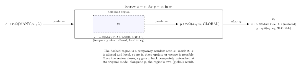
BORROWtyping rule :borrow x = e1 for y = e2 in e3“borrows” the result of evaluating a value with a fixedMANYaffinity (its uniqueness and locality, , , are unconstrained) as long as is in scope.xisaliasedi.e. cannot be updated as it is no longer unique in as well aslocalto . After is evaluated, ’s mode is restored to its original (MANY, , ) triple. ’s own result is bound toyat ( , ,GLOBAL). The third component ofy’s mode triple must beglobalbecause it must be able to survive past the end of the borrowed region.e3then gets bothx(restored to its full original mode, including its original locality) andy.
The REUSE rule #
This rule has
associated with a UNIQUE and GLOBAL space-credit i.e. a
unique location in the heap. Any two other global values,
and
, can
use this space to construct a pair type
with mode
GLOBAL. The requirement for both
and
to be global values is
because if they were local, they would be local to a region on the stack. If that
region were to no longer exist, the heap would have a reference to now-absent
value in memory.
The Algorithmic VAR: locks accumulated across closures #
OxCaml’s type inference algorithm can infer all types and modes in a program.
Modes are inferred by a constraint solver whose workings are laid out in the next section. The mode constraints that are needed for
this inference cannot be generated based on the typing rules shown so far
because the LAM rule uses locks acting on modes in
which are still
being inferred for other bindings in it.
A variable can be captured through several nested lambdas as in this fragment:
# let x = 10 in
  let g = fun z ->
    let f = fun y -> y + x in
    f z
  in
  g 5;;
- : int = 15
The variable accumulates one lock per nesting level in the context:
Γ ::= ∅ | Γ,x:- | Γ,x:τ@μ | Γ,🔒μ
and only when it’s actually referenced within a closure
does VAR sweep up all the intervening locks at once by the following rule:
The Affinity axis: The first inequality’s RHS is a meet (∧) over
and every intervening lock’s own affinity. Here
is the affinity of the
captured variable,
is the affinity of the closure and there can be i
intervening levels between where x is defined and where it is called via
capture in a context
.
On the two-element chain/two-value mode axis, MANY < ONCE,
the meet or greatest lower bound of values collapses to the value on the
left side of the relation which is MANY in this case. If any of the
intervening closures (or
itself) has a MANY affinity, the entire
meet result is a MANY. This makes a1 ≤ MANY resulting in a1 = MANY
regardless of how many of the other closure affinities were marked ONCE.
# let wrapper =
    let once_val @ once = fun () -> 42 in
    let outer @ many = fun () ->
      let inner @ once = fun () -> once_val () in
      inner ()
    in
    outer ();;
Line 4, characters 35-43:
4 |       let inner @ once = fun () -> once_val () in
                                       ^^^^^^^^
Error: The value "once_val" is "once" but is expected to be "many"
       because it is used inside the function at Lines 3-5, characters 23-14
       which is expected to be "many".
5.4 gives the same output with a slightly different message layout:
Error: The value once_val is once
       but is expected to be many
         because it is used inside the function at lines 3-5, characters 23-14
         which is expected to be many.
once_val with mode once is captured by inner @ once. However, the
intervening outer @ many contributes a many affinity into the meet on
the inequality’s right-hand side alongside inner’s own once. Since
many is the bottom of the affinity order, the outcome of the meet operation
collapses to many regardless of inner’s own declared mode. once_val’s own
affinity (a1 = once) fails the check a1 ≤ many since once can never be ≤ many.
In contrast, in the following snippet, the nesting is identical to the
fragment above with only outer marked with mode once. Now the code
compiles correctly:
# let wrapper_no_many =
    let once_val @ once = fun () -> 42 in
    let outer @ once = fun () ->
      let inner @ once = fun () -> once_val () in
      inner ()
    in
    outer ();;
val wrapper_no_many : int = 42
The Uniqueness axis: For this axis, UNIQUE ≤ ALIASED. A join
operation (∨) always tilts towards the least upper bound or the higher
(upper) value in the two-element order. Here
is the captured variable’s
own uniqueness,
that of the closure itself and
is
the dagger operation performed for the affinity of each intervening closure.
The location of the dagger symbol is on the left of
, unlike in the
Locks for Closures section, where
is a
concrete, already-elaborated closure’s affinity. Here
ranges over
intervening closures whose modes may still be unresolved at
constraint-generation time. As the
function is invertible (or
a bijection between the two two-element chains), either side
of
can be the one still unknown — the solver can compute
once
is fixed, or recover
once the required
uniqueness value is fixed by
some other constraint. (This isn’t stated outright in the paper, but is a
reasonable inference given how the constraint-solving algorithm is described.)
If any intervening lock has
= MANY (so †(
) = ALIASED,
since MANY† = ALIASED) anywhere in the chain, the value of
itself
or any other ONCE locks (ONCE† = UNIQUE) is subsumed in the join. The mode
for
(the use-site/closure) is updated with the result of the join.
# let wrapper_unique_chain =
    let xs : int list @ unique = [1;2;3] in
    let outer @ many = fun () ->
      let inner @ once = fun () -> rev_append xs [] in
      inner ()
    in
    outer ();;
Line 4, characters 46-48:
4 |       let inner @ once = fun () -> rev_append xs [] in
                                                  ^^
Error: This value is "aliased"
       because it is used inside the function at Lines 3-5, characters 23-14
       which is expected to be "many".
       However, the highlighted expression is expected to be "unique".
OxCaml 5.4 additionally traces why the highlighted expression needs to be
unique, following the chain back through the list’s own :: cells (same
further-chain pattern as elsewhere in this post):
Error: This value is aliased
         because it is used inside the function at lines 3-5, characters 23-14
         which is expected to be many.
       However, the highlighted expression is expected to be unique
         because it contains (via constructor ::) the expression at line 4, characters 36-37
         which is expected to be unique
         because it is contained (via constructor ::) in the value at line 4, characters 35-45
         which is expected to be unique.
In the following snippet, outer is marked once. With no MANY modes anywhere
in the chain of closures between outer and xs, within rev_append, when
xs is called, its mode remains unique:
# let wrapper_unique_chain_no_many =
    let xs : int list @ unique = [1;2;3] in
    let outer @ once = fun () ->
      let inner @ once = fun () -> rev_append xs [] in
      inner ()
    in
    outer ();;
val wrapper_unique_chain_no_many : int list = [3; 2; 1]
The Locality axis: Values in the locality mode axis are related as
GLOBAL < LOCAL. The third inequality in the premise of VAR is
a meet (greatest lower bound) and hence the result collapses to the minimum,
GLOBAL, whenever a single
= GLOBAL appears anywhere in the chain of
closures between the captured variable with a declared locality
and
being that of the closure (the use site). A local variable
simply cannot survive being captured through a chain containing even
one global lock because as soon as the meet operation collapses to GLOBAL,
≤ GLOBAL can only hold if
= GLOBAL.
# let wrapper_local_chain =
    let xs : int list @ local = [1;2;3] in
    let outer @ global = fun () ->
      let inner @ local = fun () -> length_local xs in
      inner ()
    in
    outer ();;
Line 4, characters 49-51:
4 |       let inner @ local = fun () -> length_local xs in
                                                     ^^
Error: The value "xs" is "local" but is expected to be "global"
       because it is used inside the function at Lines 3-5, characters 25-14
which is expected to be "global".(5.4 drops the quotes and lowercases lines in the internal
reference, but is otherwise identical.)
The following snipped has outer with mode local with no GLOBAL modes
anywhere in the chain between xs being declared and called in inner.
xs reaches length_local keeping its mode local. (Note that inner () is
deliberately kept out of tail position here — a plain tail call
would hit the separate tail-call/region restriction outlined in a later section):
# let wrapper_local_chain_no_global =
    let xs : int list @ local = [1;2;3] in
    let outer @ local = fun () ->
      let inner @ local = fun () -> length_local xs in
      1 + inner ()
    in
    outer ();;
val wrapper_local_chain_no_global : int = 4
A Comment on the Modes as Qualifiers #
In section 3.1 of the paper, the following sentence makes a claim: “Systems based on type qualifiers, like Walker (David Walker. 2005. Substructural type systems. Advanced topics in types and programming languages (2005), 3–44), annotate all types with qualifiers… In contrast, our system uses qualifiers on computation types, but omits them from value types. Instead, we introduce a box type to represent the modality .”
A type system based on Walker’s pretypes supposes every type to have a qualifier with an ordering relationship required between a type container’s qualifier and its components. In contrast, the mode system presented in the paper attaches one mode to the overall typing judgment of an expression, but does not require every sub-component of a compound type to carry its own separately-annotated qualifier. The mechanics of how the OxCaml constraint solver resolves the inequalities generated by VAR, together with the other type judgments is laid out in the next section.
The Mechanics of Mode Inference #
Inference variables and positive/negative mode expressions #
Mode expressions are extended with inference variables (α), both for triples
denoting entire modes and for each individual axis. In BNF format:
Positive mode expressions (a⁺,u⁺,l⁺) and negative mode
expressions (a⁻,u⁻,l⁻) are defined per mode axis in BNF format as follows:
Positive expressions form using a join (∨) which is the least upper bound of
its components while negative expressions are formed using a meet (∧) or greatest
lower bound of its components. The dagger operation (and its inverse) lets a
negative expression on one axis contribute a positive expression on the other
axis (affinity/uniqueness) (examples of this were seen in the Algorithmic
Var section.)
The following mode expression relations:
, , , ,
are solved by taking the transitive closure of all such relations.
In the above grammar,
is the base mode to be inferred. After every
constituent in a chain of mode relations resolves to a concrete value, the
result is a meet or a join, computed on each mode axis’s two-element chain
with MANY<ONCE, UNIQUE<ALIASED, GLOBAL<LOCAL. Both meet and join, as lattice
operations, are associative — join always collapses toward the greatest value
on an axis, meet toward the least
Let’s look at an example:
# let rec rev_append xs acc =
    match xs with
    | [] -> acc
    | (x :: rest) -> rev_append rest (x :: acc);;
val rev_append : 'a list -> 'a list -> 'a list = <fun>

# let xs_1 : int list @ unique = [1;2;3;4;5] in
  let f = fun ls -> rev_append xs_1 ls in
  let a = f [6] in
  let b = f [7] in
  (a, b);;
- : int list * int list = ([5; 4; 3; 2; 1; 6], [5; 4; 3; 2; 1; 7])
Every unannotated mode slot above is a fresh inference variable. rev_append’s
own type has three of them, one per argument/result position:
with (and likewise for , ) each a fully free triple; no rule generates a constraint of the shape against any of their components.
f’s two unannotated LAM slots are likewise fresh:
Since f is applied twice (f [6] and f [7]), the solver derives
But because
is never constrained by anything in rev_append’s
definition, no algorithmic VAR inequality of the form
is ever generated at all — there is
no rule producing a relation between
(or
) and xs_1’s own
ascription.
Adding a @ unique ascription to rev_append:
# let rec rev_append xs acc : _ list @ unique =
    match xs with
    | [] -> acc
    | (x :: rest) -> rev_append rest (x :: acc);;
val rev_append : 'a list @ unique -> 'a list @ unique -> 'a list @ unique =
  <fun>

# let xs_1 : int list @ unique = [1;2;3;4;5] in
  let f = fun ls -> rev_append xs_1 ls in
  let a = f [6] in
  let b = f [7] in
  (a, b);;
Line 4, characters 8-9:
4 | let b = f [7] in
            ^
Error: This value is used here,
       but it is defined as once and has already been used:
Line 3, characters 8-9:
3 | let a = f [6] in
            ^
Modifying rev_append with an @ unique ascription, the same inference proceeds differently. Its
uniqueness components are now pinned by the explicit annotation:
f’s two LAM slots still start out fresh, exactly as before:
But now the accumulated-lock uniqueness inequality from the algorithmic
VAR rule is no longer vacuous. Capturing xs_1 (itself
)
through f’s lock
generates:
Substituting the now-known concrete values ( , ), and since joining with the bottom of the uniqueness chain is the identity:
UNIQUE is the bottom of its axis, so the only value
is UNIQUE itself — forcing
, and since
is a bijection (
):
This directly conflicts with the separate constraint calling f twice
would otherwise impose:
needed for a second reference to f to coexist with the first —
and
are incompatible, which is
exactly why the rejection occurs.
Let’s go over another example where positive and negative mode expressions are involved.
A positive (synthesized) expression:
# let rec rev_append xs acc : _ list @ unique =
    match xs with
    | [] -> acc
    | (x :: rest) -> rev_append rest (x :: acc);;

# let wrapper_unique_chain =
    let xs : int list @ unique = [1;2;3] in
    let outer @ many = fun () ->
      let inner @ once = fun () -> rev_append xs [] in
      inner ()
    in
    outer ();;
Line 4, characters 46-48:
4 |       let inner @ once = fun () -> rev_append xs [] in
                                                  ^^
Error: This value is "aliased"
       because it is used inside the function at Lines 3-5, characters 23-14
       which is expected to be "many".
       However, the highlighted expression is expected to be "unique".
xs is captured through two nested closures, so both inner’s and
outer’s locks accumulate:
Capturing xs through both locks generates the accumulated-lock
uniqueness inequality:
The left side here is a positive expression that is built via join operations
from modes that are known (xs’s own UNIQUE, and the daggered
affinities of both locks already crossed). Substituting concrete values
(
, the bottom, contributes nothing;
, the top, absorbs everything):
forcing . The entire left-hand side was assembled bottom-up from what’s already given, exactly matching the grammar shape: .
A negative (required) expression:
# let wrapper =
    let once_val @ once = fun () -> 42 in
    let outer @ many = fun () ->
      let inner @ once = fun () -> once_val () in
      inner ()
    in
    outer ();;
Line 4, characters 35-43:
4 |       let inner @ once = fun () -> once_val () in
                                       ^^^^^^^^
Error: The value "once_val" is "once" but is expected to be "many"
       because it is used inside the function at Lines 3-5, characters 23-14
       which is expected to be "many".
The accumulated-lock affinity inequality is:
The right side,
, is a negative
expression that is built via meet. It matches the rule:
. It is not synthesized
from once_val’s mode value(s) but it is the ceiling
once_val is required to fit under given the modes of the closures already
entered around it. Substituting concrete values:
Since MANY < ONCE, ONCE is not ≤ MANY — the inequality fails, and
once_val is rejected specifically because of outer’s contribution to
this constructed ceiling.
The following quick-reference calculations are always helpful for reducing long chains of joins and meets:
Meet (negative expressions — collapses toward the axis minimum/lower bound):
| expression | collapses to |
|---|---|
a⁻ = a₁∧a₂∧... |
MANY the instant any aᵢ=MANY, ONCE only if every aᵢ=ONCE |
u⁻ = u₁∧u₂∧... |
UNIQUE the instant any uᵢ=UNIQUE, ALIASED only if every uᵢ=ALIASED |
l⁻ = l₁∧l₂∧... |
GLOBAL the instant any lᵢ=GLOBAL, LOCAL only if every lᵢ=LOCAL |
Join (positive expressions — collapses toward the axis maximum/upper bound):
| expression | collapses to |
|---|---|
a⁺ = a₁∨a₂∨... |
ONCE the instant any aᵢ=ONCE, MANY only if every aᵢ=MANY |
u⁺ = u₁∨u₂∨... |
ALIASED the instant any uᵢ=ALIASED, UNIQUE only if every uᵢ=UNIQUE |
l⁺ = l₁∨l₂∨... |
LOCAL the instant any lᵢ=LOCAL, GLOBAL only if every lᵢ=GLOBAL |
The form for the relations specified earlier:
, , , ,
can be made sense by taking an example for the affinity mode axis:
a⁺ |
a⁻ |
holds? |
|---|---|---|
| MANY | MANY | ✓ |
| MANY | ONCE | ✓ |
| ONCE | ONCE | ✓ |
| ONCE | MANY | ✗ |
The a⁺ inference variable accumulates a lower bound (the join of every “the
variable value must at least be” requirement on the variable) whereas
a⁻ accumulates an upper bound (the meet of every “the variable must at most
this be” requirement). a⁺ ≤ a⁻ is the check that a value satisfying both
actually exists i.e. if the
accumulated lower bound were to exceed the accumulated upper bound, the
requirements would be contradictory (“crossed”). The same calculations apply to
the other points in the mode triple with u⁺≤ u⁻ and l⁺≤ l⁻.
Solving by transitive closure #
Working out how the transitive closure of modes is easier done with actual values. The rules for lattices are: join is a least upper bound and meet a greatest lower bound, so in any lattice:
where are all elements in a set that forms a lattice.
Applying both rules repeatedly, an n-element join on the left of a⁺≤ a⁻
against an m-element meet on the right splits into the full n×m cross
product of atomic pairwise constraints. For example:
Flattened by associativity, the joins on the left have 3 leaves (MANY, α₁,α₂), the meets on the right have 3 (α₃, α₄, α₅`), which makes this so
constraint splits into 3×3 = 9 atomic constraints:
MANY is the affinity axis minimum, so the whole top row with MANY ≤ any variable is trivially true no matter what α₃/α₄/α₅ resolve to which is how those three edges
carry no information and can be dropped. Had the atom been ONCE, ONCE ≤ x
would force x = ONCE for each and then propagate the update to the other
constraints. Remaining constraints are:
Building a graph of these ≤
edges, then taking its transitive closure (x≤y, y≤z ⟹ x≤z) and rejecting
any edge/path that forces a value below the axis minimum or above the axis
maximum (e.g. a path forcing ONCE≤MANY) is how the entire set of constraints
is narrowed down and solved.
The shared-node reading of α.
As per the grammar in mode inference, the rules:
share no same-axis production
by e.g. letting a⁻ sit inside a⁺. Only the dagger operator crosses axes
where affinity
a⁺ can embed a uniqueness u⁻ for example.
But the same α that does show up on both sides of the whole constraint set (not within one constraint’s own tree) is a
shared graph node linking two separate atomic constraints e.g.:
Transitive closure composes C1 and C2 through the shared node α
into a new derived edge:
α never “becomes” positive or negative depending on which side it’s
written on as it’s one node with edges pointing in (from C1 above) and out
(to C2 above). The transitive closure is when an edge points in and an edge
points out of a relation, we add the direct edge across both. This is
substitution-by-closure (propagating a resolved bound through a shared
variable across separate constraints), and not substitution-by-grammar,
simply because the a⁺/a⁻ BNF refers to calculated modes, not the ones
written in the code.
# let chain_weaken_ok =
    let producer : int list @ unique = [1; 2; 3] in
    let mid = producer in
    let consumer : int list @ aliased = mid in
    consumer;;
val chain_weaken_ok : int list = [1; 2; 3]
The code above is a working example on the uniqueness axis (UNIQUE < ALIASED). mid is left
unannotated: it is the shared inference variable α, a bridge between a producer site and a consumer site.
mid’s own inferred mode is the shared node α. producer’s @ unique
annotation supplies an edge into α (a lower bound), and consumer’s
@ aliased annotation supplies an edge out of α (an upper bound it
must feed):
Closure chains these through the shared node α into the derived fact
which holds, so any mode α resolves to is in the proper order for the affinity
mode.
Now if the example is changed to:
# let chain_weaken_fails =
    let producer : int list @ aliased = [1; 2; 3] in
    let mid = producer in
    let consumer : int list @ unique = mid in
    consumer;;
Line 4, characters 39-42:
4 |     let consumer : int list @ unique = mid in
                                           ^^^
Error: This value is "aliased" but is expected to be "unique".mid’s own inferred mode is again the shared node α. producer’s
@ aliased annotation supplies an edge into α (a lower bound), and
consumer’s @ unique annotation supplies an edge out of α (an
upper bound it must feed):
Closure chains these through the shared node α into the derived fact
which does not hold as it is the reverse of the required order UNIQUE ≤ ALIASED. Now the compiler correctly rejects it even though mid itself is still just passed straight through unchanged.
Problems with the Typing Rules #
The paper lists the following problems with the rules making up the type system described in the sub-sections of Type system Rules:
- In the
LAMrule, locks act on the modes in Γ. However, at the time the lock operation takes place, the values of the modes needed may yet need inferring. - The
SUBrule is not syntax-directed. - The context joining operation (
+) is non-deterministic when used to split a context
The algorithmic VAR rule and the related details laid out in
the previous two sections (The Mechanics of Mode
Inference, Solving by Transitive
Closure) help solve the first problem.
Before looking at how the second problem is tackled, let’s first see how a context-splitting operation can be made deterministic and resolves the third issue.
Context splitting #
Context splitting is the dual operation to context
joining. The declarative type rules
seen up until now (except for the algorithmic VAR rule, which isn’t part of this declarative rule set at all) pick contexts
in their premises Γ₁, Γ₂ nondeterministically. In a rule with Γ₁ + Γ₂ = Γ,
both Γ₁, Γ₂ are chosen to make Γ suitable for the typing rule. The typing rules do
not specify how Γ₁, Γ₂ are to be chosen i.e. what should Γ₁, Γ₂
contain in order for Γ to make the rule sound. The rules specified in
Appendix B of the paper replaces the earlier rules with ones that are
parameterised by the free variables of the two subterms actually
being checked.
(The paper denotes this operation with its own custom Y-shaped glyph with hooked
arrowheads on the two upper arms; split is used here in its place since that
glyph has no standard font support.)
Γ_X keeps Γ’s bindings only for variables in X, blanking the rest to
x:-. The same holds in Γ_Y. This separation is what makes the split
deterministic for any variable that is not in the free variable set.
Variables in the relevant free-variable set keep their full,
correct binding from Γ so all expressions containing them can be type-checked
while everything else is blanked with -, making it unavailable.
The following equations are the counterparts of the join (+) operations
(denoted by J here)
explained in the section on joining
usages:
- A:
split(∅) = ∅+∅↔︎ J1:∅+∅ = ∅ - B:
split(Γ,🔒μ) = Γ_X,🔒μ + Γ_Y,🔒μ↔︎ (no counterpart in J1..J5). Locks were not part of context syntax where+was defined (They were added only after the algorithmicVARrule was defined). A lock is copied unchanged to both contextsXandY. - C:
split(Γ,x:-) = Γ_X,x:- + Γ_Y,x:-↔︎ J2:(Γ1,x:-)+(Γ2,x:-) = (Γ1+Γ2),x:-An unused variable stays unused in both contexts, since it isn’t a free variable of eitherXorY - D:
split(Γ,x:τ@μ) = Γ_X,x:τ@μ + Γ_Y,x:-wherex ∈ X, x ∉ Y↔︎ J3:(Γ1,x:τ@μ)+(Γ2,x:-) = (Γ1+Γ2),x:τ@μ— J3 merges the same variable across contexts (with use and without use) into actual use in the resulting context. This rule D prises open that combination to returnxto the side that actually needs it (X, sincex∈FV(e1)) and marks the other side asx:-. - E:
split(Γ,x:τ@μ) = Γ_X,x:- + Γ_Y,x:τ@μwherex∉X, x∈Y↔︎ J4:(Γ1,x:-)+(Γ2,x:τ@μ) = (Γ1+Γ2),x:τ@μ— a mirror of the previous rule. - F:
split(Γ,x:τ@(a,u,l)) = Γ_X,x:τ@(a,aliased,l) + Γ_Y,x:τ@(a,aliased,l)wherea≤many, x∈X, x∈Y↔︎ J5:(Γ1,x:τ@(_,aliased,l))+(Γ2,x:τ@(_,aliased,l)) = (Γ1+Γ2),x:τ@(many,_,l)requiresaliasedon both inputs and producesmanyaffinity on the output. This rule requiresa≤manyon input (sincemanyis the axis minimum, soa≤manyliterally forcesa=many) and producesaliasedon bothx’s in the output. F’s precondition is the guarantee provided by J5 as output and F’s output is the input needed by J5 i.e. the rules are inversions. This explains why a variable needed by both subterms at once can only ever be handed out as two aliased copies and that uniqueness cannot be duplicated, aliased values can.
A point that should be carefully noted: The x:- notation is used in multiple
sections of the paper with different meanings which are:
- Context
-(in all the sections above and until section 4 of the paper): static. The meaning of “x:-” is thatxhas no free occurrence. The binding may still be alive elsewhere inΓbut is absent from the current context. Calculating the free variables of an expressione(FV(e)) will either help find a binding or keep it blank. - Store
-(Section 4 of the paper): “x:-” denotes thatxwas accessed at a mode requiring exclusivity and is now consumed. This state can be arrived at by tracking what expressions have been evaluated so far.
The typing rules that actually need the split operation in their premises
are: APP, PAIR, SPLIT, LET, CASE, REUSE, BORROW. All the other
rules - VAR, SUB, LAM, UNIT, INL, INR, BOX, UNBOX have zero or
just one premise.
The syntax-directed CASE rule (from Figure 11 in the paper) is:
CASE only needs one split (Γ1 for
e1 and Γ2 for the branches), not a three-way split like in the
REUSE/BORROW rules:
This is why rules like PAIR or BORROW need to actually split their contexts
(two for PAIR, three for BORROW) so that the subterms in the resulting
contexts can meet the genuine simultaneous access or aliasing requirements.
Syntax-directed BOX/UNBOX rules #
Figure 12 of the paper specializes the original typing rules BOX/UNBOX
to the syntax-directed versions for the three concrete modalities A, M, G:
Original rules:
A note: Initially I found these rules to be unintuitive and hard to read. Only afer constructing examples did the following become clear:
BOXrule: an expressionehas a mode which denotes a mode to which a modality is applied perhaps changing one or more of its axes. The result is a boxed value where the outer box’s mode never changes. The contents inside the box have their mode set to (as described in the section on BOX/UNBOX). The entire expressioneis said to be boxed with modality .UNBOXrule: Here the expressioneis the result from theBOXrule and the type/mode denotes the larger “box” or structure within which the original expression was put viaBOX. The mode pertains to only this larger box. Wheneis unboxed, the result is i.e. the mode of the original boxed expression is recovered via using the modality applied to the mode of the entire box .
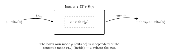
Figure 12 from the paper shows several variants of these BOX/UNBOX rules
with free variables. The submoding (SUB) rule is also silently used to resolve
problem (2). The rules are as follows:
M-box
Expression e is boxed with a many affinity whereas a (the affinity for the
box itself) can be any value. Modes u, l remain unchanged.
M-unbox (the box holding the many-forced content)
The affinity
(for the box itself) is either many or once. When e is
unboxed, the affinity
can be set to anything (
=
either many or once is fine as MANY is a sub-mode of ONCE). Modes u, l remain unchanged.
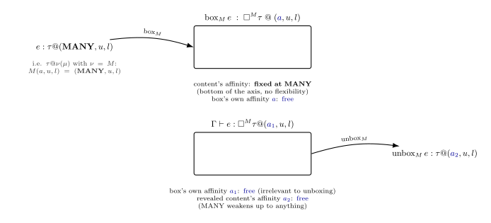
Making
free means the compiler doesn’t need a separate step to figure out
when to apply the SUB rule. It is already built into the unboxing
rule itself making the above operation stay within a single step over the
syntax unlike an alternate system where SUB has to be applied after unboxing.
A-box
The uniqueness
for the expression e can be either unique or
aliased. After boxing with modality A, the box itself can have any value for
. Modes a
and l are unchanged.
A-unbox
When unboxing a box with any uniqueness, the resulting uniqueness for e is
ALIASED. Modes a, l are unchanged. This means that if a boxed expression
at unique mode were unboxed,
for the unboxed expression would only be
aliased.
Together, A-box and A-unbox show that a box’s own uniqueness (
/
in A-box, u in A-unbox) is entirely independent of what it forces on its
content: the box itself can be unique or aliased freely, but the A
modality always forces the content to aliased on unboxing, regardless of
what the box’s own mode was.
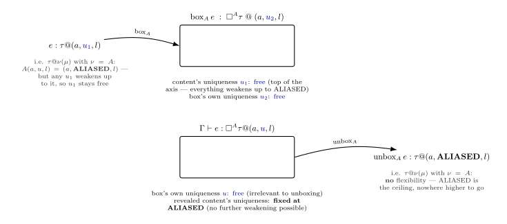
Here the SUB rule is folded as follows: after unboxing, a term having the uniqueness
mode ALIASED means it is being extracted from a boxed value where the term was
either a unique value or an aliased value. If it was unique, then it can
be used as an aliased result and if it was aliased, then the mode after
unboxing is the same.
G-box
Both
and a can be any value but expression e must be global for the
boxing to occur. The boxed expression carries a through unchanged, while claiming a fresh, independent value for uniqueness (u2) and locality (l).
G-unbox
The boxed expression is unboxed to ALIASED with a unchanged from the
premise and a new value for
independent of the one for the boxed term
.
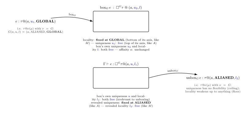
The SUB rules work here as follows: An expression boxed with mode axis global
within a larger expression of any locality l, when unboxed will return an
aliased value. This makes sense in terms of taking a global value and
putting it in a box; when that value comes out, it is aliased leaving locality
free to be either global or local. If
is claimed as global (matching what
it truly was before boxing), no subsumption is required. If it is local, then
the mode is at the upper end of the axis and so here SUB eventually
subsumes a global value to local mode.
Notes on Surface-Language Design Decision - Regions and Tail Calls #
Leaving a region is an operation that occurs during run time when a function call returns to its
parent region and for which the compiler runtime system has to move a stack pointer to
reclaim the region’s memory. This directly conflicts with a native optimization
in OCaml — tail-calls. When a function a calls another function b in a tail position,
a’s (the calling function) stack-frame is reused by b (the called function). If the
function in the tail position is recursive, it repeatedly uses the same
stack-frame. (If a programmer specifically wants to stack-allocate a
value in the current region and pass it to a call in tail position instead, they
have to annotate that call to explicitly suppress the tail-call optimization.)
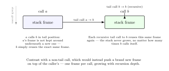
If any values within a are local, b reusing a’s frame means values
local to a would be lost before the call to b is even made. Such a restriction on values local to a region would block most
tail-recursive
functions from accepting parameters with local mode in the first place. For
this, OxCaml has a fourth locality mode, regional, defined as:
The semantics of regional are not documented in the paper but a quick check
via Claude for the mode in the compiler source (typing/mode_intf.mli) turned
up a dedicated Regionality module with type t = Global | Regional | Local
matching the above order. However this 3-valued axis is kept separate from the
simpler 2-valued Locality axis (Local/Global) exposed on arrow types.
So regional only exists in the fuller internal representation, with explicit
conversions like regional_to_local and regional_to_global bridging the two.
A regional value is one that may escape only as far as the current region.
This lets a function like iter accept a local argument f, treat it as
regional inside its own body, and safely pass it along to a tail call but only
if iter’s own definition says so. Annotating f’s type with @ local makes
iter’s own region able to carry a local closure across every tail-recursive
call within it:
# let rec iter (f @ local) l =
    match l with
    | [] -> ()
    | a :: l -> f a; iter f l;;
val iter : ('a -> 'b) @ local -> 'a list -> unit = <fun>

# let f @ local = fun x -> print_int x; print_char ' ' in
  iter f [1;2;3];;
1 2 3 - : unit = ()![Diagram of iter’s tail-recursive frame reuse: each call f a is a genuinely separate, non-tail call that pushes and pops its own small frame, but the surrounding iter f l call is a tail call, so it keeps reusing the exact same iter frame across every element of the list until [] -> () ends the recursion.](../assets/images/iter-tailcall-diagram.svg)
Leaving the @ local annotation off iter’s own parameter changes the output.
Without it, iter’s inferred type defaults to requiring f to be global and
now passing a local f is rejected outright:
# let rec iter f l =
    match l with
    | [] -> ()
    | a :: l -> f a; iter f l;;
val iter : ('a -> 'b) -> 'a list -> unit = <fun>

# let f @ local = fun x -> print_int x; print_char ' ' in
  iter f [1;2;3];;
Line 2, characters 5-6:
2 |   iter f [1;2;3];;
         ^
Error: This value is "local" but is expected to be "global".
In the above example, what if l were a local value created inside another
function? When that function call ended, its stack frame would be reclaimed,
and so would the allocated value of l. In that case, an OxCaml command exclave_ would let l
escape its local region through a tail position to its parent function call.
A concrete example: a function make_list builds a local list and returns it via
exclave_ so it does survive past make_list’s own region. The returned
l is then passed into the iter f l function call. And this example
needs one more annotation than the previous one: the list parameter also has
to be marked @ local, not just f:
# let rec iter (f @ local) (l @ local) =
    match l with
    | [] -> ()
    | a :: l -> f a; iter f l;;
val iter : ('a @ local -> 'b) @ local -> 'a list @ local -> unit = <fun>

# let make_list n = exclave_ (List.init n (fun i -> i + 1));;
val make_list : int -> int list @ local = <fun>

# let f @ local = fun x -> print_int x; print_char ' ' in
  let l = make_list 3 in
  iter f l;;
1 2 3 - : unit = ()
exclave_ must sit in tail position of the current region i.e. nothing can
happen after it before the function returns. Binding its result to a let
and doing something with it first (rather than returning it immediately)
breaks that requirement outright:
# let make_list_fails n =
    let doubled = exclave_ (List.init n (fun i -> i + 1)) in
    List.length doubled |> ignore;
    doubled;;
Line 2, characters 18-57:
2 |     let doubled = exclave_ (List.init n (fun i -> i + 1)) in
                      ^^^^^^^^^^^^^^^^^^^^^^^^^^^^^^^^^^^^^^^
Error: Exclave expression should only be in tail position of the current region.
Note iter’s inferred type now also shows f’s own argument as 'a @ local
since l’s elements come from a local list, each element a pattern-matched
out of it is itself local, so f must be able to accept a local argument too.
Credits and Wrapping up #
This post took a while to come up with but using Claude as a tool was helpful in many ways. I used it to come up with most of the code snippets, check the text for errors of grammar, ensure that the content from the paper reproduced here (the type inference equations) is correct, generate the (SVG) diagrams and finally make sure that all the code samples ran correctly.
Apart from a brief discussion on how the mode system handles uniqueness as compared to a system with pre-types, I haven’t added anything related to the variety of how different language systems conceptualize and deal with linear values and/or unique values. Section 8.1 of the paper has a wealth of references for that. An additional paper that has been very well-written and which ties together the idea of combining linearity with uniqueness is Linearity and Uniqueness: An Entente Cordiale.
Sections 4 and 5 still remain to be put up as posts. Here’s hoping that I get to work through them not too far off from now.
Links/References #
- Oxidizing OCaml with Modal Memory Management
- Get OxCaml
- Boxing and unboxing values in OCaml
- For Fitch-Style Modal logics: